Iris interactive

This script demonstrates interactive plotting the Iris dataset using matplotlib.

• 
• 
• 
• 
• 
• 
• 
• 
• 
• 
• 
• 
• 
• 
• 
• 

/Users/sravya/venv/lib/python3.9/site-packages/NNSOM/plots.py:1209: RankWarning: Polyfit may be poorly conditioned
  m, p = np.polyfit(x[neuron], y[neuron], 1)
start training
end training

from NNSOM.plots import SOMPlots
from NNSOM.utils import *

import numpy as np
from numpy.random import default_rng
import matplotlib.pyplot as plt

from sklearn.datasets import load_iris
from sklearn.linear_model import LogisticRegression

import os

# SOM Parameters
SOM_Row_Num = 4  # The number of row used for the SOM grid.
Dimensions = (SOM_Row_Num, SOM_Row_Num)  # The dimensions of the SOM grid.

# Training Parameters
Epochs = 500
Steps = 100
Init_neighborhood = 3

# Random State
SEED = 1234567
rng = default_rng(SEED)

# Data Preparation
iris = load_iris()
X = iris.data
y = iris.target

# Preprocessing data
X = X[rng.permutation(len(X))]
y = y[rng.permutation(len(X))]

# Determine model dir and file name
model_dir = os.path.abspath(os.path.join(os.getcwd(), "..", "..", "..", "..", "Model"))
Trained_SOM_File = "SOM_Model_iris_Epoch_" + str(Epochs) + '_Seed_'  + str(SEED) + '_Size_' + str(SOM_Row_Num) + '.pkl'

# Load som instance
som = SOMPlots(Dimensions)
som = som.load_pickle(Trained_SOM_File, model_dir + os.sep)

# Data Processing
clust, dist, mdist, clustSize = som.cluster_data(X)

# Items for int_dict
num1 = get_cluster_array(X[:, 0], clust)
num2 = get_cluster_array(X[:, 1], clust)
cat = count_classes_in_cluster(y, clust)

# Items for plots
perc_sentosa = get_perc_cluster(y, 0, clust)
iris_class_counts_cluster_array = count_classes_in_cluster(y, clust)
align = np.arange(len(iris_class_counts_cluster_array[0]))
num_classes = count_classes_in_cluster(y, clust)
num_sentosa = num_classes[:, 0]

int_dict = {
        'data': X,
        'target': y,
        'clust': clust,
        'num1': num1,
        'num2': num2,
        'cat': cat,
        'topn': 5,
    }

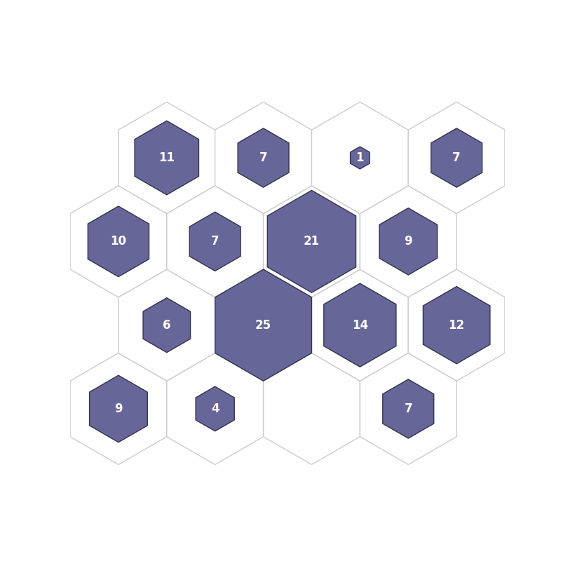
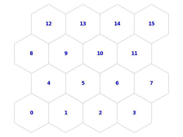
# Interactive hit hist
fig, ax, patches, text = som.hit_hist(X, mouse_click=True, **int_dict)
plt.show()

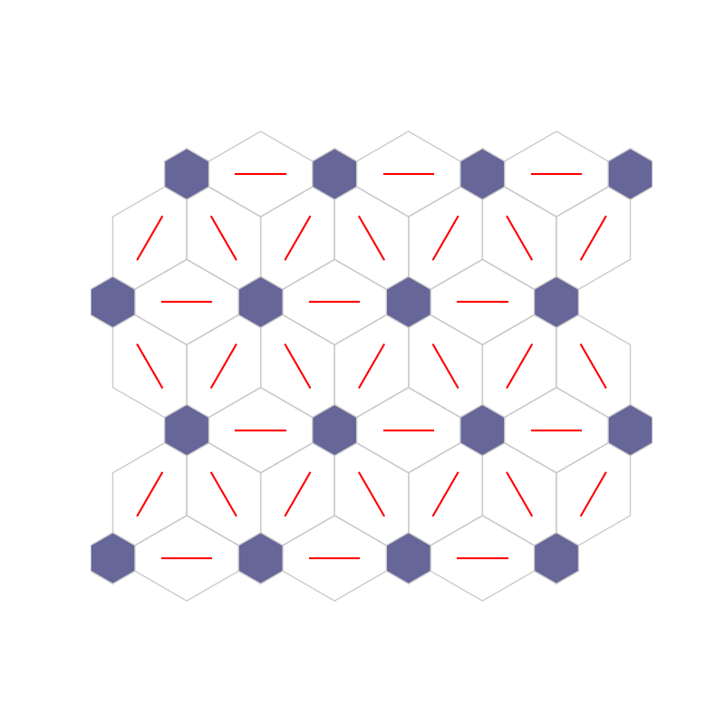
# Interactive neuron dist
fig, ax, patches = som.neuron_dist_plot(True, **int_dict)
plt.show()

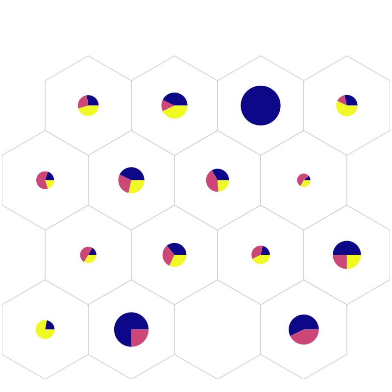
# Interactive pie plot
fig, ax, h_axes = som.plt_pie(iris_class_counts_cluster_array, perc_sentosa, mouse_click=True, **int_dict)
plt.show()

# Interactive plt_top
fig, ax, patches = som.plt_top(True, **int_dict)
plt.show()

# Interactive plt_top_num
fig, ax, patches, text = som.plt_top_num(True, **int_dict)
plt.show()

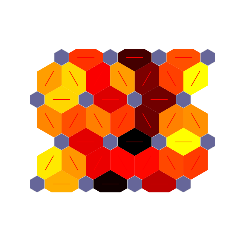
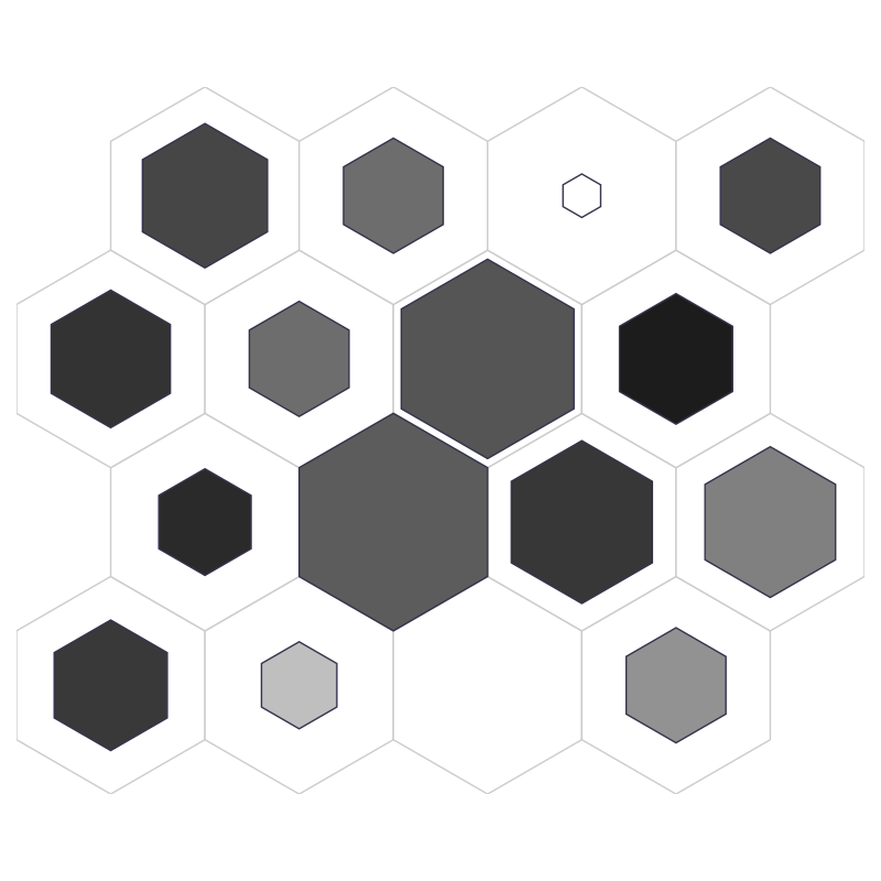
# Interactive gray plot
fig, ax, patches, text = som.gray_hist(X, perc_sentosa, True, **int_dict)
plt.show()

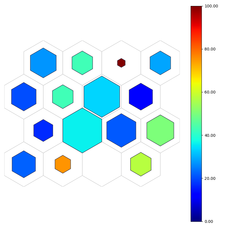
# Interactive color plot
fig, ax, patches, text, cbar = som.color_hist(X, perc_sentosa, True, **int_dict)
plt.show()

# Interactive plt_nc
fig, ax, patches = som.plt_nc(True, **int_dict)
plt.show()

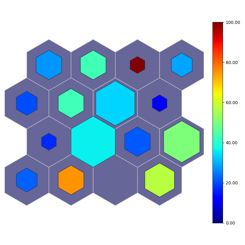
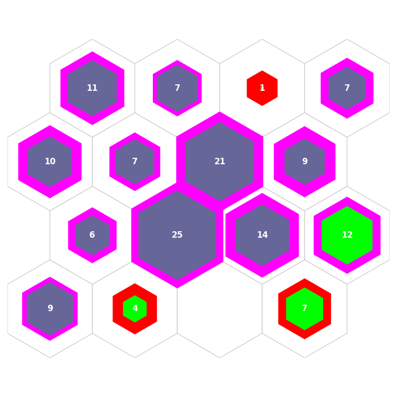
# interactive simple grid
fig, ax, patches, cbar = som.simple_grid(perc_sentosa, num_sentosa, True, **int_dict)
plt.show()

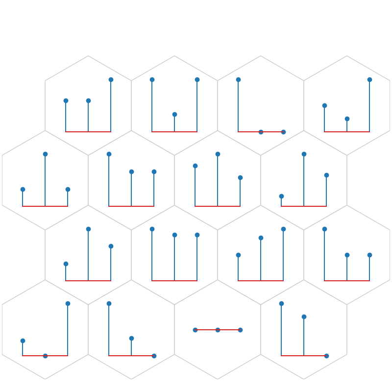
# interactive stem plot
fig, ax, h_axes = som.plt_stem(align, iris_class_counts_cluster_array, True, **int_dict)
plt.show()

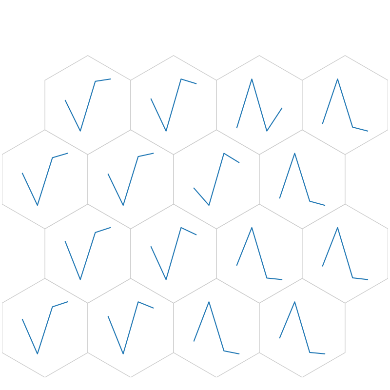
# interactive line plot
fig, ax, h_axes = som.plt_wgts(True, **int_dict)
plt.show()

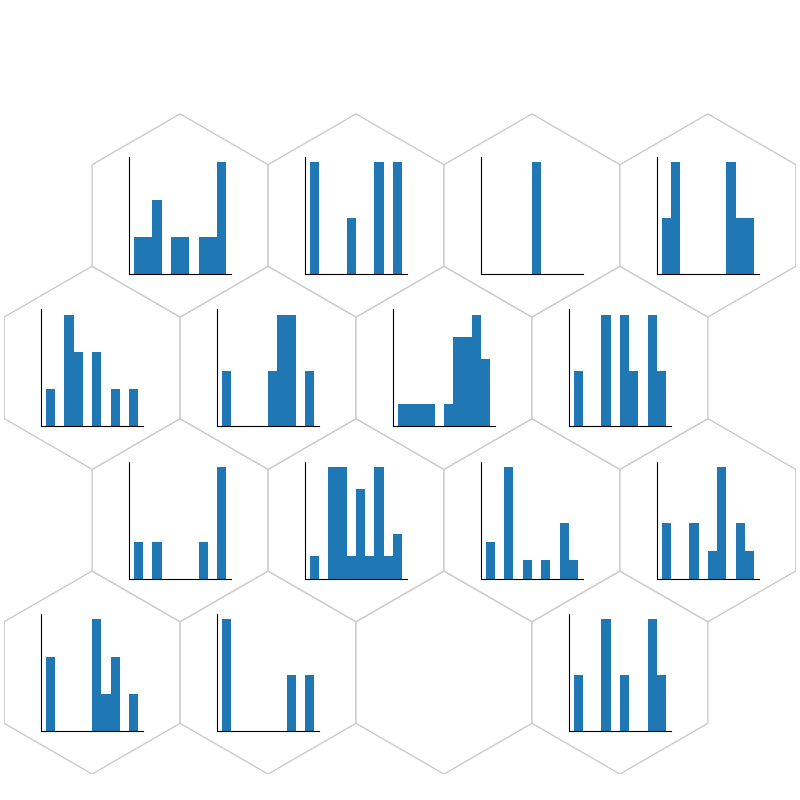
# Interactive Histogram
fig, ax, h_axes = som.plt_histogram(num1, True, **int_dict)
plt.show()

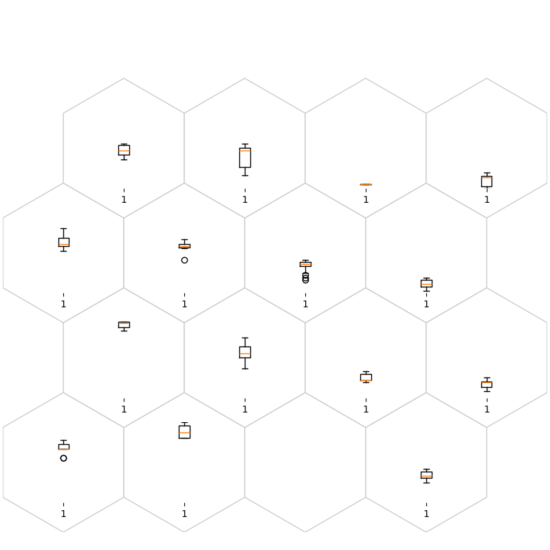
# Interactive Boxplot
fig, ax, h_axes = som.plt_boxplot(num1, True, **int_dict)
plt.show()

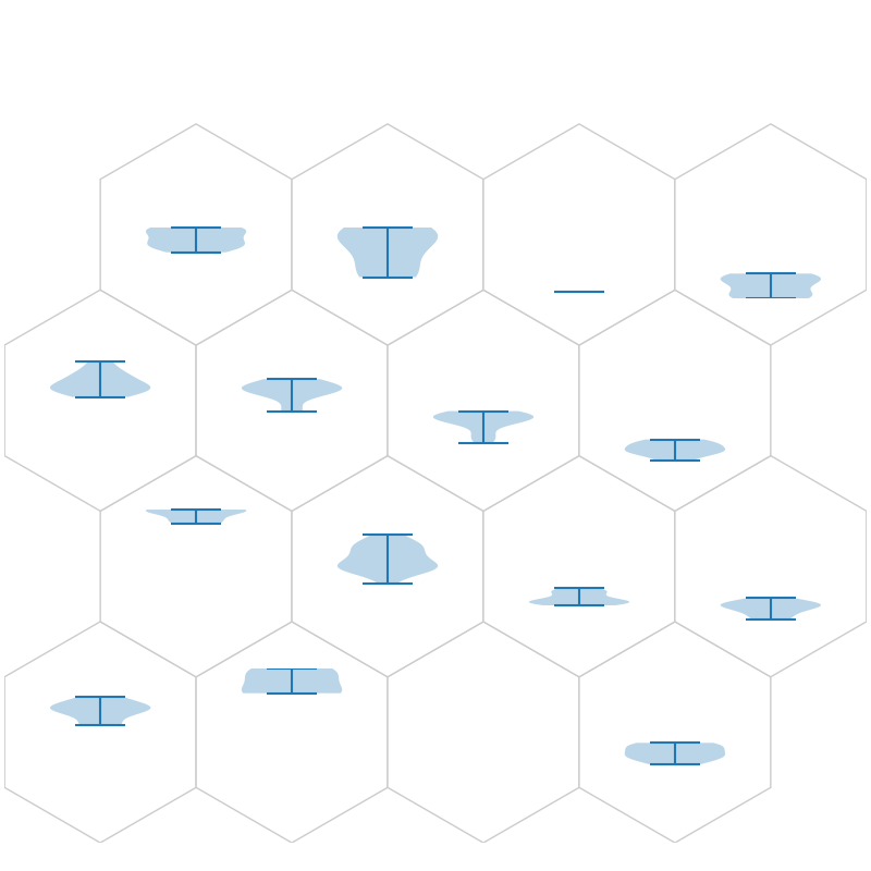
# Interactive Violin Plot
fig, ax, h_axes = som.plt_violin_plot(num1, True, **int_dict)
plt.show()

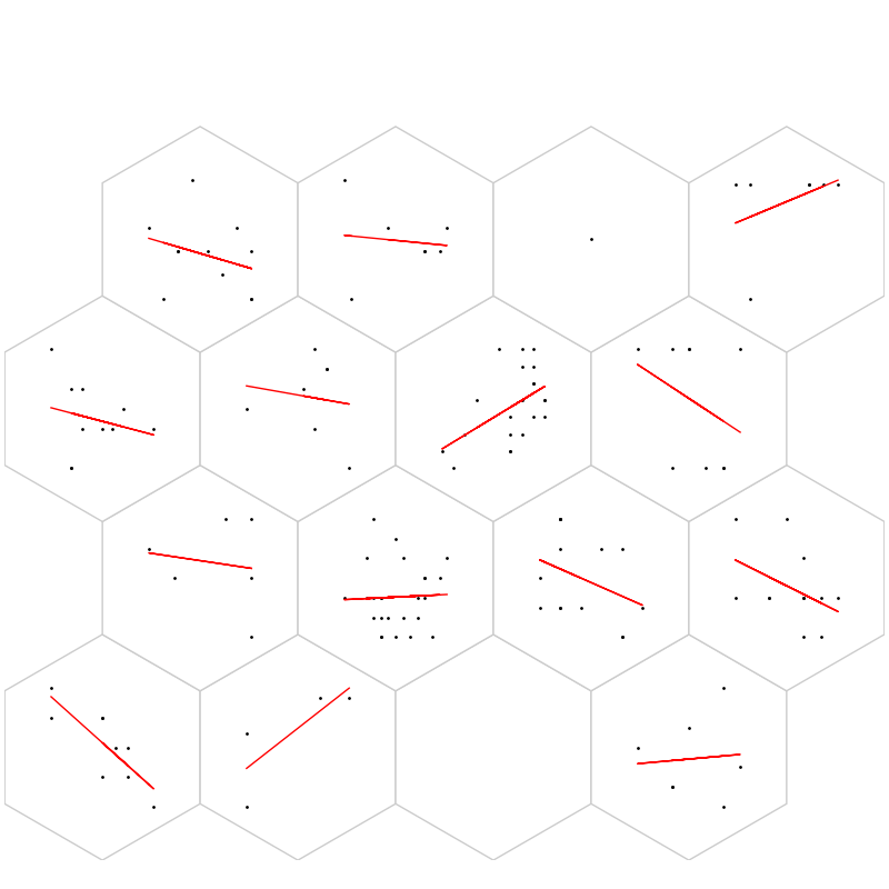
# Interactive Scatter plot
fig, ax, h_axes = som.plt_scatter(num1, num2, True, True, **int_dict)
plt.show()

# Train Logistic Regression on Iris
print('start training')
logit = LogisticRegression(random_state=SEED)
logit.fit(X, y)
results = logit.predict(X)
print('end training')

ind_missClass = get_ind_misclassified(y, results)
tp, ind21, fp, ind12 = get_conf_indices(y, results, 0)

if 'clust' in int_dict:
    del int_dict['clust']

fig, ax, patches, text = som.cmplx_hit_hist(X, clust, perc_sentosa, ind_missClass, ind21, ind12, mouse_click=True,
                                            **int_dict)
plt.show()