Iris plot

This script demonstrates plotting the Iris dataset using matplotlib.

• 
• 
• 
• 
• 
• 
• 
• 
• 
• 
• 
• 
• 
• 
• 
• 
• 

/Users/sravya/venv/lib/python3.9/site-packages/NNSOM/plots.py:1196: RankWarning: Polyfit may be poorly conditioned
  m, p = np.polyfit(x[neuron], y[neuron], 1)
/Users/sravya/venv/lib/python3.9/site-packages/NNSOM/plots.py:1196: RankWarning: Polyfit may be poorly conditioned
  m, p = np.polyfit(x[neuron], y[neuron], 1)

from NNSOM.plots import SOMPlots

from numpy.random import default_rng
import matplotlib.pyplot as plt

from sklearn.datasets import load_iris
from sklearn.preprocessing import MinMaxScaler

import os

# Random State
SEED = 1234567
rng = default_rng(SEED)

# Data Preprocessing
iris = load_iris()
X = iris.data
y = iris.target
X = X[rng.permutation(len(X))]
y = y[rng.permutation(len(X))]
scaler = MinMaxScaler(feature_range=(-1, 1))

# Define the directory path for saving the model outside the repository
model_dir = os.path.abspath(os.path.join(os.getcwd(), "..", "..", "..", "..", "Model"))
trained_file_name = "SOM_Model_iris_Epoch_500_Seed_1234567_Size_4.pkl"

# SOM Parameters
SOM_Row_Num = 4  # The number of row used for the SOM grid.
Dimensions = (SOM_Row_Num, SOM_Row_Num) # The dimensions of the SOM grid.

som = SOMPlots(Dimensions)
som = som.load_pickle(trained_file_name, model_dir + os.sep)

# Data Preparation for Visualization
clust, dist, mdist, clustSize = som.cluster_data(X)

data_dict = {
    "data": X,
    "target": y,
    "clust": clust
}

# Visualization
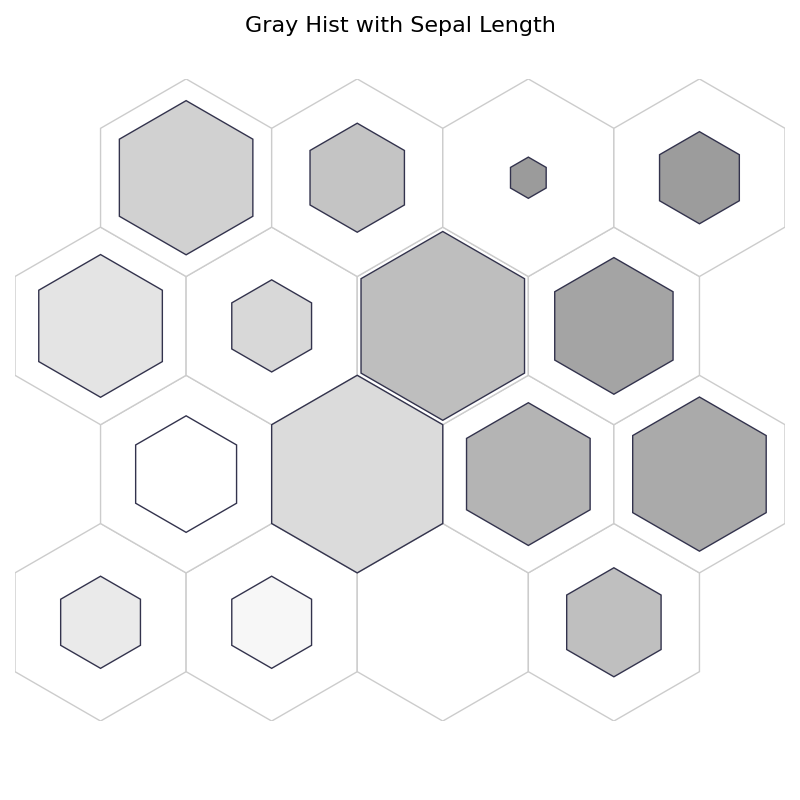
# Grey Hist
fig, ax, pathces, text = som.plot('gray_hist', data_dict, ind=0)
plt.suptitle("Gray Hist with Sepal Length", fontsize=16)
plt.show()

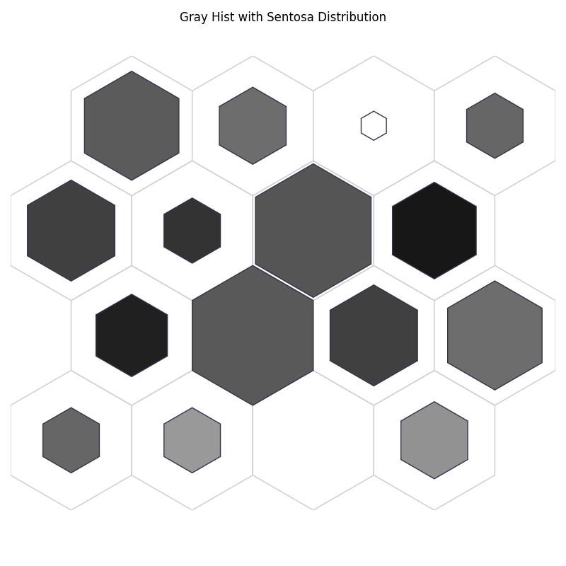
fig, ax, pathces, text = som.plot('gray_hist', data_dict, target_class=0)
plt.suptitle("Gray Hist with Sentosa Distribution")
plt.show()

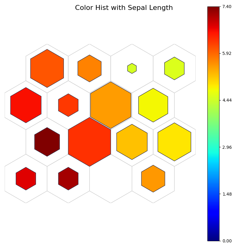
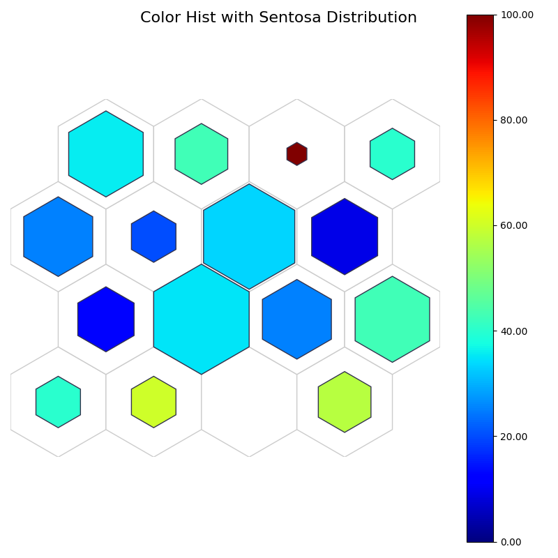
# Color Hist
fig, ax, pathces, text, cbar = som.plot('color_hist', data_dict, ind=0)
plt.suptitle("Color Hist with Sepal Length", fontsize=16)
plt.show()

fig, ax, patches, text, cbar = som.plot('color_hist', data_dict, target_class=0)
plt.suptitle("Color Hist with Sentosa Distribution", fontsize=16)
plt.show()

# Pie Chart
fig, ax, h_axes = som.plot("pie", data_dict)
plt.suptitle("Iris Class Distribution", fontsize=16)
plt.show()

# Stem Plot
fig, ax, h_axes = som.plot('stem', data_dict)
plt.show()

# Histogram
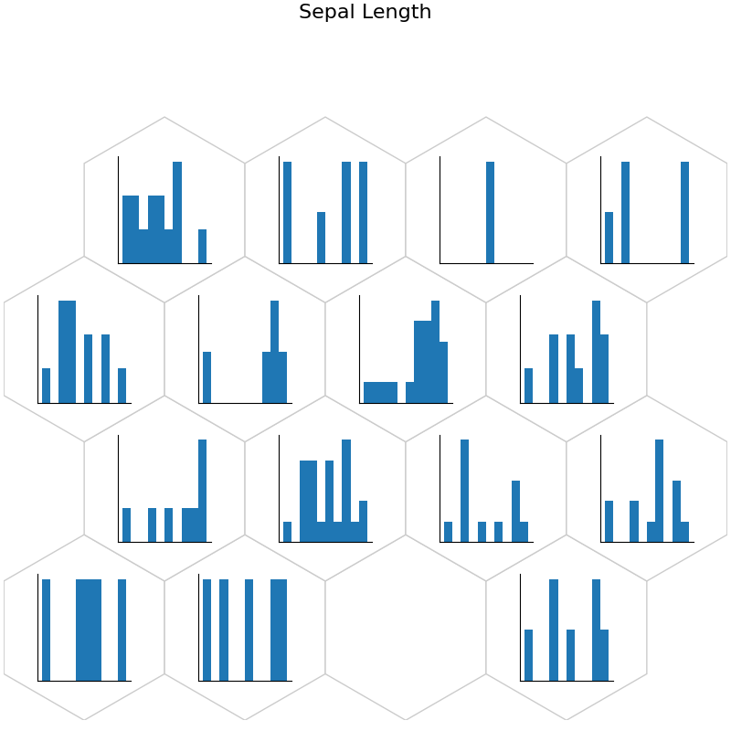
fig, ax, h_axes = som.plot('hist', data_dict, ind=0)
plt.suptitle("Sepal Length", fontsize=16)
plt.show()

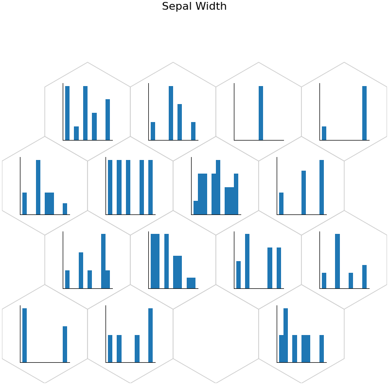
fig, ax, h_axes = som.plot('hist', data_dict, ind=1)
plt.suptitle("Sepal Width", fontsize=16)
plt.show()

# Boxplot
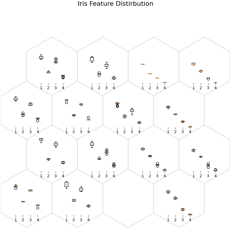
fig, ax, h_axes = som.plot("box", data_dict)
plt.suptitle("Iris Feature Distirbution", fontsize=16)
plt.show()

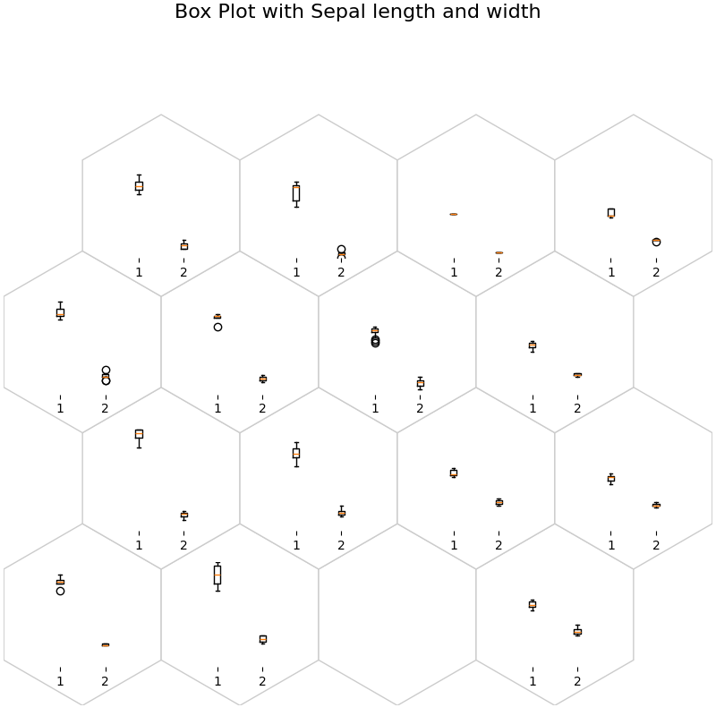
fig, ax, h_axes = som.plot("box", data_dict, ind=[0, 1])
plt.suptitle("Box Plot with Sepal length and width", fontsize=16)
plt.show()

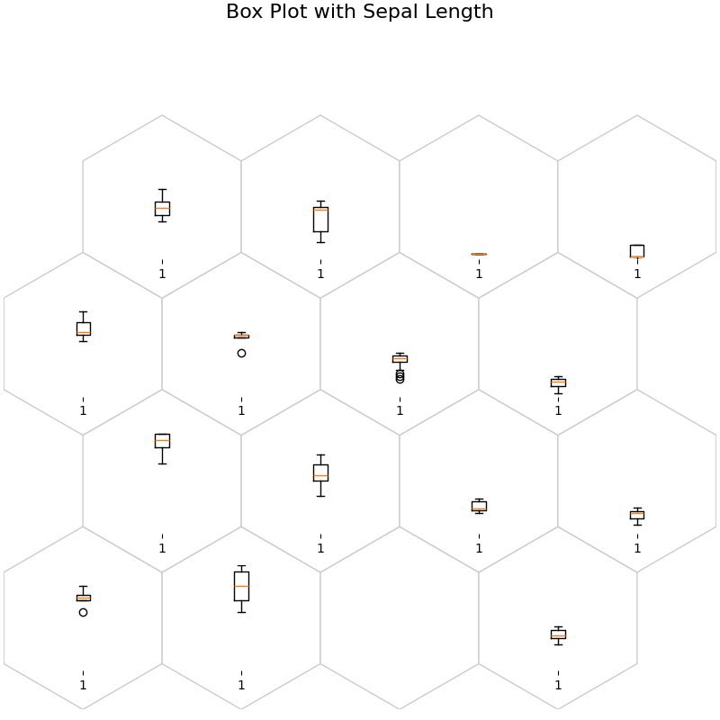
fig, ax, h_axes = som.plot("box", data_dict, ind=0)
plt.suptitle("Box Plot with Sepal Length", fontsize=16)
plt.show()

# Violin plot
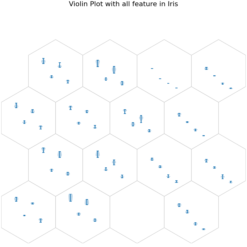
fig, ax, h_axes = som.plot("violin", data_dict)
plt.suptitle("Violin Plot with all feature in Iris", fontsize=16)
plt.show()

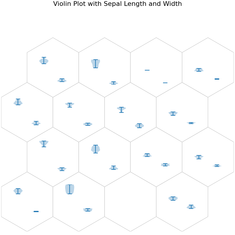
fig, ax, h_axes = som.plot("violin", data_dict, ind=[0, 1])
plt.suptitle("Violin Plot with Sepal Length and Width", fontsize=16)
plt.show()

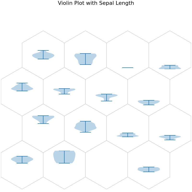
fig, ax, h_axes = som.plot("violin", data_dict, ind=0)
plt.suptitle("Violin Plot with Sepal Length", fontsize=16)
plt.show()

# Scatter Plot
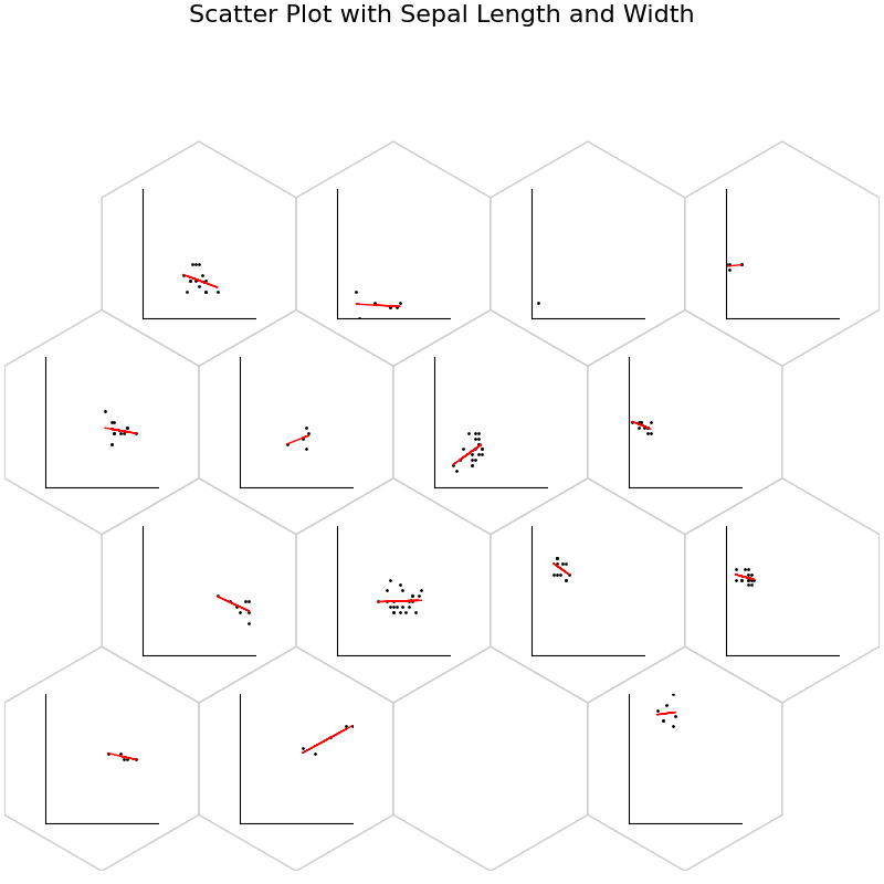
fig, ax, h_axes = som.plot("scatter", data_dict, ind=[0, 1])
plt.suptitle("Scatter Plot with Sepal Length and Width", fontsize=16)
plt.show()

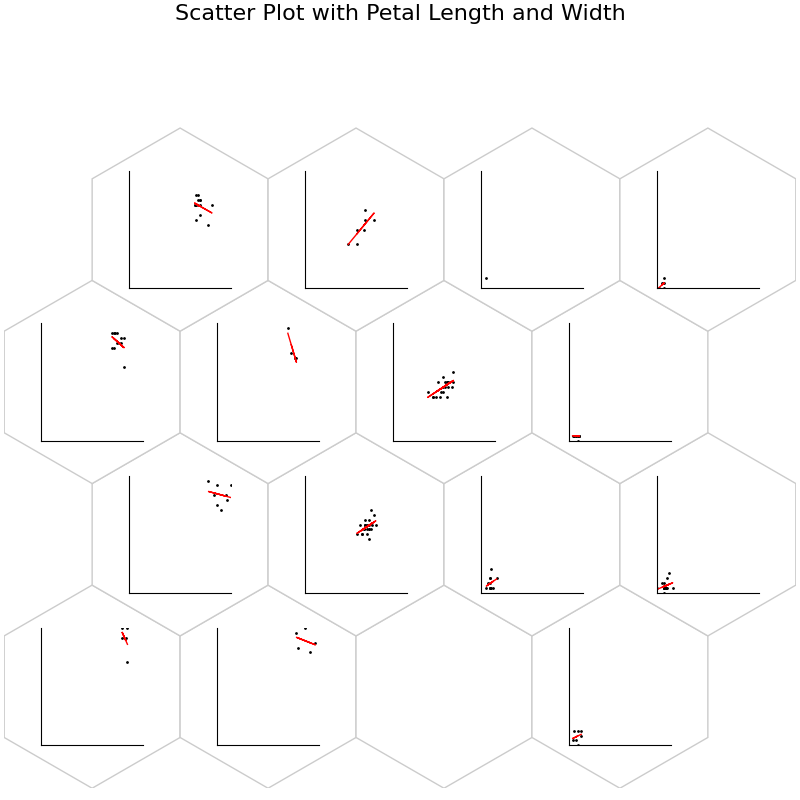
fig, ax, h_axes = som.plot("scatter", data_dict, ind=[2, 3])
plt.suptitle("Scatter Plot with Petal Length and Width", fontsize=16)
plt.show()

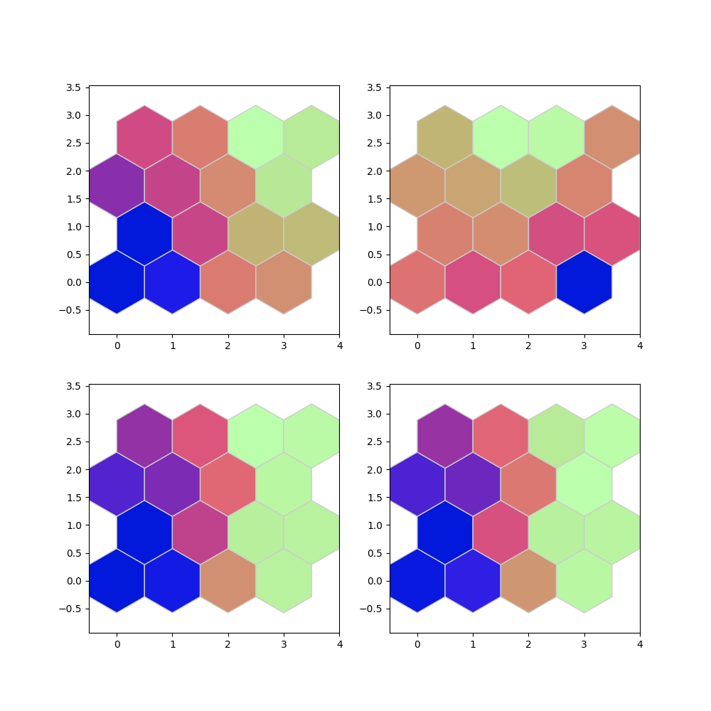
# Components Plane
som.plot('component_planes', data_dict)